numpy.random.Generator.binomial

method

random.Generator.binomial(n, p, size=None)

Draw samples from a binomial distribution.

Samples are drawn from a binomial distribution with specified parameters, n trials and p probability of success where n an integer >= 0 and p is in the interval [0,1]. (n may be input as a float, but it is truncated to an integer in use)

Parameters:

nint or array_like of ints

Parameter of the distribution, >= 0. Floats are also accepted, but they will be truncated to integers.

pfloat or array_like of floats

Parameter of the distribution, >= 0 and <=1.

sizeint or tuple of ints, optional

Output shape. If the given shape is, e.g., (m, n, k), then m * n * k samples are drawn. If size is None (default), a single value is returned if n and p are both scalars. Otherwise, np.broadcast(n, p).size samples are drawn.

Returns:

outndarray or scalar

Drawn samples from the parameterized binomial distribution, where each sample is equal to the number of successes over the n trials.

See also

scipy.stats.binom

probability density function, distribution or cumulative density function, etc.

Notes

The probability density for the binomial distribution is

\[P(N) = \binom{n}{N}p^N(1-p)^{n-N},\]

where \(n\) is the number of trials, \(p\) is the probability of success, and \(N\) is the number of successes.

When estimating the standard error of a proportion in a population by using a random sample, the normal distribution works well unless the product p*n <=5, where p = population proportion estimate, and n = number of samples, in which case the binomial distribution is used instead. For example, a sample of 15 people shows 4 who are left handed, and 11 who are right handed. Then p = 4/15 = 27%. 0.27*15 = 4, so the binomial distribution should be used in this case.

References

[1]

Dalgaard, Peter, “Introductory Statistics with R”, Springer-Verlag, 2002.

[2]

Glantz, Stanton A. “Primer of Biostatistics.”, McGraw-Hill, Fifth Edition, 2002.

[3]

Lentner, Marvin, “Elementary Applied Statistics”, Bogden and Quigley, 1972.

[4]

Weisstein, Eric W. “Binomial Distribution.” From MathWorld–A Wolfram Web Resource. https://mathworld.wolfram.com/BinomialDistribution.html

[5]

Wikipedia, “Binomial distribution”, https://en.wikipedia.org/wiki/Binomial_distribution

Examples

Draw samples from the distribution:

>>> rng = np.random.default_rng()
>>> n, p, size = 10, .5, 10000  
>>> s = rng.binomial(n, p, 10000)

Assume a company drills 9 wild-cat oil exploration wells, each with an estimated probability of success of p=0.1. All nine wells fail. What is the probability of that happening?

Over size = 20,000 trials the probability of this happening is on average:

>>> n, p, size = 9, 0.1, 20000
>>> np.sum(rng.binomial(n=n, p=p, size=size) == 0)/size
0.39015  # may vary

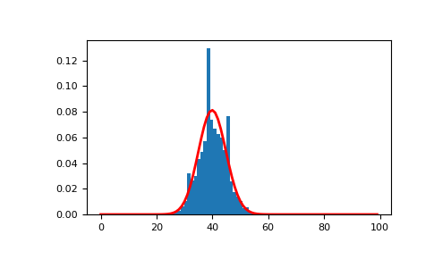
The following can be used to visualize a sample with n=100, p=0.4 and the corresponding probability density function:

>>> import matplotlib.pyplot as plt
>>> from scipy.stats import binom
>>> n, p, size = 100, 0.4, 10000
>>> sample = rng.binomial(n, p, size=size)
>>> count, bins, _ = plt.hist(sample, 30, density=True)
>>> x = np.arange(n)
>>> y = binom.pmf(x, n, p)
>>> plt.plot(x, y, linewidth=2, color='r')