numpy.percentile#
- numpy.percentile(a, q, axis=None, out=None, overwrite_input=False, method='linear', keepdims=False, *, weights=None)[source]#
Compute the q-th percentile of the data along the specified axis.
Returns the q-th percentile(s) of the array elements.
- Parameters:
- aarray_like of real numbers
Input array or object that can be converted to an array.
- qarray_like of float
Percentage or sequence of percentages for the percentiles to compute. Values must be between 0 and 100 inclusive.
- axis{int, tuple of int, None}, optional
Axis or axes along which the percentiles are computed. The default is to compute the percentile(s) along a flattened version of the array.
- outndarray, optional
Alternative output array in which to place the result. It must have the same shape and buffer length as the expected output, but the type (of the output) will be cast if necessary.
- overwrite_inputbool, optional
If True, then allow the input array a to be modified by intermediate calculations, to save memory. In this case, the contents of the input a after this function completes is undefined.
- methodstr, optional
This parameter specifies the method to use for estimating the percentile. There are many different methods, some unique to NumPy. See the notes for explanation. The options sorted by their R type as summarized in the H&F paper [1] are:
‘inverted_cdf’
‘averaged_inverted_cdf’
‘closest_observation’
‘interpolated_inverted_cdf’
‘hazen’
‘weibull’
‘linear’ (default)
‘median_unbiased’
‘normal_unbiased’
The first three methods are discontinuous. NumPy further defines the following discontinuous variations of the default ‘linear’ (7.) option:
‘lower’
‘higher’,
‘midpoint’
‘nearest’
Changed in version 1.22.0: This argument was previously called “interpolation” and only offered the “linear” default and last four options.
- keepdimsbool, optional
If this is set to True, the axes which are reduced are left in the result as dimensions with size one. With this option, the result will broadcast correctly against the original array a.
- weightsarray_like, optional
An array of weights associated with the values in a. Each value in a contributes to the percentile according to its associated weight. The weights array can either be 1-D (in which case its length must be the size of a along the given axis) or of the same shape as a. If weights=None, then all data in a are assumed to have a weight equal to one. Only method=”inverted_cdf” supports weights. See the notes for more details.
Added in version 2.0.0.
- Returns:
- percentilescalar or ndarray
If q is a single percentile and axis=None, then the result is a scalar. If multiple percentiles are given, first axis of the result corresponds to the percentiles. The other axes are the axes that remain after the reduction of a. If the input contains integers, the output data-type is
float64. Otherwise, the output data-type is the same as that of the input. If out is specified, that array is returned instead.
See also
meanmedianequivalent to
percentile(..., 50)nanpercentilequantileequivalent to percentile, except q in the range [0, 1].
Notes
The behavior of
numpy.percentilewith percentage q is that ofnumpy.quantilewith argumentq/100. For more information, please seenumpy.quantile.References
[1]R. J. Hyndman and Y. Fan, “Sample quantiles in statistical packages,” The American Statistician, 50(4), pp. 361-365, 1996
Examples
>>> import numpy as np
>>> a = np.array([[10, 7, 4], [3, 2, 1]])
>>> a
array([[10,  7,  4],
       [ 3,  2,  1]])
>>> np.percentile(a, 50)
3.5
>>> np.percentile(a, 50, axis=0)
array([6.5, 4.5, 2.5])
>>> np.percentile(a, 50, axis=1)
array([7.,  2.])
>>> np.percentile(a, 50, axis=1, keepdims=True)
array([[7.],
       [2.]])
>>> m = np.percentile(a, 50, axis=0)
>>> out = np.zeros_like(m)
>>> np.percentile(a, 50, axis=0, out=out)
array([6.5, 4.5, 2.5])
>>> m
array([6.5, 4.5, 2.5])
>>> b = a.copy()
>>> np.percentile(b, 50, axis=1, overwrite_input=True)
array([7.,  2.])
>>> assert not np.all(a == b)
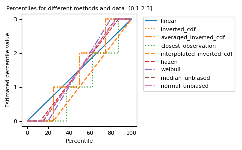
The different methods can be visualized graphically:
import matplotlib.pyplot as plt

a = np.arange(4)
p = np.linspace(0, 100, 6001)
ax = plt.gca()
lines = [
    ('linear', '-', 'C0'),
    ('inverted_cdf', ':', 'C1'),
    # Almost the same as `inverted_cdf`:
    ('averaged_inverted_cdf', '-.', 'C1'),
    ('closest_observation', ':', 'C2'),
    ('interpolated_inverted_cdf', '--', 'C1'),
    ('hazen', '--', 'C3'),
    ('weibull', '-.', 'C4'),
    ('median_unbiased', '--', 'C5'),
    ('normal_unbiased', '-.', 'C6'),
    ]
for method, style, color in lines:
    ax.plot(
        p, np.percentile(a, p, method=method),
        label=method, linestyle=style, color=color)
ax.set(
    title='Percentiles for different methods and data: ' + str(a),
    xlabel='Percentile',
    ylabel='Estimated percentile value',
    yticks=a)
ax.legend(bbox_to_anchor=(1.03, 1))
plt.tight_layout()
plt.show()